Objectives: Topics
Objectives: Goals
Theorem 7.37. Singular Value Decomposition.
Let
\(A\) be an
\(m\times n\) matrix with rank
\(r\text{.}\) Then
\(A\) can be written as
\begin{equation*}
A = U\Sigma V^T = \begin{bmatrix} \vec u_1 \amp \cdots \amp \vec u_m \end{bmatrix} \begin{bmatrix} \sigma_1 \amp 0 \amp 0 \amp \cdots \amp 0 \\ 0 \amp \sigma_2 \amp 0 \amp \cdots \amp 0 \\ \vdots \amp \vdots \amp \ddots \amp \vdots \amp \vdots \\ 0 \amp 0 \amp \cdots \amp \sigma_r \amp 0 \\ 0 \amp 0 \amp \cdots \amp 0 \amp 0 \end{bmatrix}\begin{bmatrix} \vec v_1^T \\ \vdots \\ \vec v_n^T \end{bmatrix}
\end{equation*}
-
\(U\) is an \(m\times m\) orthogonal matrix,
-
\(V\) is an \(n\times n\) orthogonal matrix,
-
\(\Sigma\) is an \(m\times n\) diagonal matrix with diagonal entries \(\sigma_1,\dots,\sigma_r\text{,}\) where \(\sigma_1 \geq \sigma_2 \geq \cdots \geq \sigma_r \gt 0\text{.}\)
Note that Singular Value Decomposition applies to
any matrix, not just symmetric or square matrices.
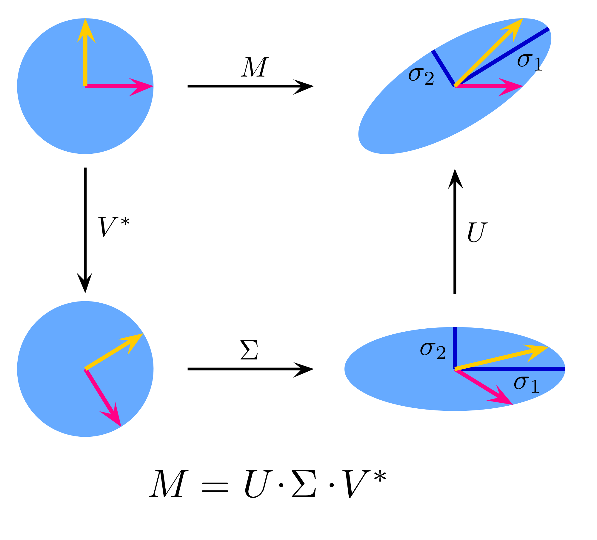
Recall from
Theorem 6.34 that multiplication by an orthogonal matrix does not change the angles between vectors nor the vector’s length. Therefore, if
\(U\) is an orthogonal matrix, we have that the linear transformation
\(T(\vec x) = U\vec x\) must simply be a rotation and/or reflection.
Note that multiplication by a
\(m \times n\) diagonal matrix
\(\Sigma\) changes the vector from being in
\(\mathbb{R}^n\) to being in
\(\mathbb{R}^m\text{,}\) and then scales it along the appropriate coordinate axes.
Therefore, in general, we can use the SVD of a matrix
\(A\) to describe how the linear transformation
\(T(\vec x) = A\vec x\) acts on the vectors in
\(\mathbb{R}^n\text{.}\)
Example 7.40.
\begin{equation*}
A = \begin{bmatrix}3 \amp 8 \\ 0 \amp 3 \end{bmatrix}.
\end{equation*}
Example 7.41.
\begin{equation*}
A=\begin{bmatrix}1 \amp -1\\ -2 \amp 2\\ 2 \amp -2\end{bmatrix}.
\end{equation*}
The SVD has been applied to many modern applications in CS, engineering, and mathematics. Some applications are:
-
Constructing bases for the four fundamental subspaces
-
Forming approximations of a matrix
-
Estimating the rank and the condition number of a matrix
-
Computing the pseudoinverse of a matrix
-
Linear least-squares problems
-
Non-linear least-squares problems
-
Image compression
-
Machine learning and data mining
-
Facial Recognition
-
Principal component analysis
Students are expected to be familiar with the first two items. We will explore these two items below.
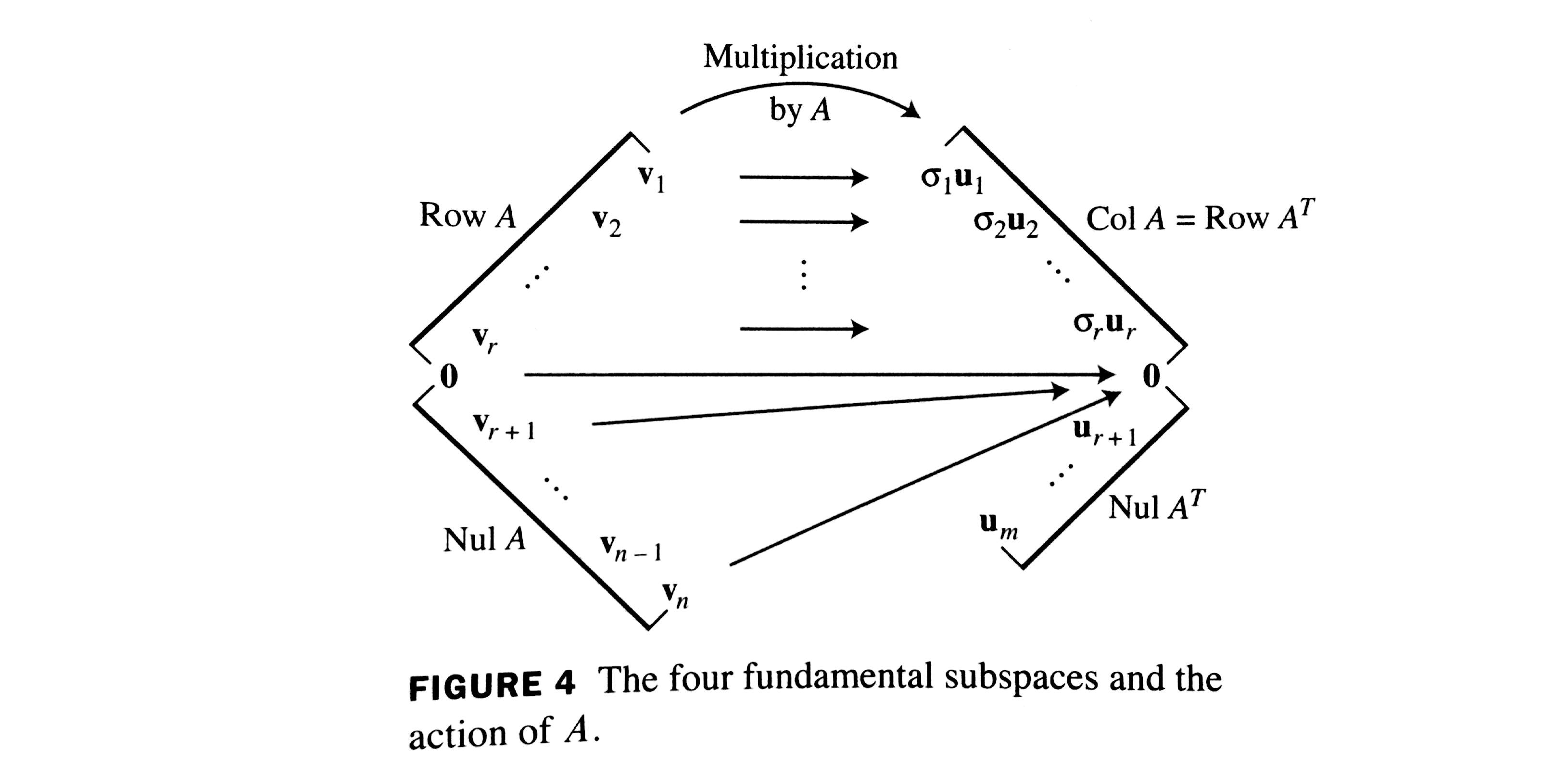
Let
\(A = U\Sigma V^T\) be an
\(m \times n\) matrix with rank
\(r\text{.}\)
Consider the columns of \(U\text{:}\)
-
Recall that the formula for calculating the first few columns of \(U\) is
\begin{equation*}
\vec u_i = \dfrac{1}{\sigma_i}A\vec v_i\text{.}
\end{equation*}
-
It follows that
\(\left\{\vec u_1, \dots, \vec u_r\right\}\) is a set of
\(\underline{\hspace{2in}}\) vectors that all live in
\(\underline{\hspace{1.5in}}\text{.}\)
-
Therefore, the first
\(r\) columns of
\(U\) form an
\(\underline{\hspace{3in}}\) for
\(\underline{\hspace{1.5in}}\)
-
Since the remaining columns of
\(U\) are created so that all columns of
\(U\) form an orthonormal basis for
\(\mathbb{R}^m\text{,}\) we see that
\(\left\{\vec u_{r+1}, \dots, \vec u_m\right\}\) is a set of
\(\underline{\hspace{2in}}\) vectors which live in
\(\underline{\hspace{3in}}\text{.}\)
-
Therefore, the last
\(m - r\) columns of
\(U\) form an
\(\underline{\hspace{3in}}\) for
\(\underline{\hspace{1.5in}}\text{.}\)
Now, consider the rows of \(V^T\text{:}\)
-
The last
\(n-r\) rows of
\(V^T\) are eigenvectors of
\(A^TA\) which correspond to an eigenvalue of
\(\underline{\hspace{1in}}\text{.}\)
-
Therefore,
\(\left\{\vec v_{r+1}, \dots, \vec v_n\right\}\) form an
\(\underline{\hspace{3in}}\) for
\(\underline{\hspace{2in}}\text{.}\)
-
We have that
\(\Nul(A^TA) = \Nul(A)\text{.}\) Thus, the last
\(n - r\) rows of
\(V^T\) form an
\(\underline{\hspace{3in}}\) for
\(\underline{\hspace{1.5in}}\text{.}\)
-
Since
\(V^T\) is an orthogonal matrix, we know that it’s
\(n\) rows form an orthonormal basis for
\(\mathbb{R}^n\text{.}\) Therefore,
\(\left\{\vec v_1, \dots, \vec v_r\right\}\) is a set of
\(\underline{\hspace{2in}}\) vectors which live in
\(\underline{\hspace{3in}}\text{.}\)
-
It follows that the first
\(r\) rows of
\(V^T\) form an
\(\underline{\hspace{3in}}\) for
\(\underline{\hspace{1.5in}}\text{.}\)
We end this section, and this course, by investigating the connection between Spectral Decomposition and Image Compression. Consider an image in grayscale consisting of pixels in a
\(880 \times 1100\) grid. Since each pixel is in grayscale, we can assign it an integer value between 0 and 255 depending on how gray it is, where 0 is black and 255 is white. We can form a
\(880 \times 1100\) matrix where each entry is the grayscale value of the associated pixel. In general, the rank of this matrix could be quite high.
For example, suppose we have selected an image and created the associated matrix and it has rank
\(776\text{.}\) One way to store this image in a slightly compressed manner is to store the
\(776\) basis vectors for
\(\Col(A)\text{,}\) and then store a list of linear combinations describing how to use these
\(776\) vectors to recreate all
\(880\) columns (the dimensions of an image are reversed, first horizontal, then vertical).
Question 7.46.
Could we compress the file size further? Suppose we were okay with a little error in our image. Perhaps just a hair of fuzziness that could be corrected open reopening the compressed file. How could we go about doing this?
The idea is to find a good enough approximation of the image. We can use Spectral Decomposition to find the best rank
\(j\) approximation for
\(j = 1, \dots, r\text{.}\) We can save tons of storage by letting
\(j\) be small, but then our image will be super blurry. We can have a very accurate image by letting
\(j\) be large, but then the compression’s filesize is not much smaller than the original’s filesize. We need to find a
\(j\) which balances these, a good approximation with small filesize.
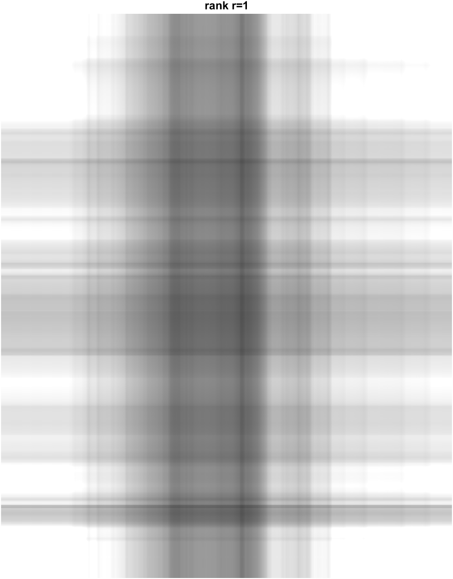
Here is the best rank 1 approximation for the image. Can you tell what the image is?
Proceed through the next few images slowly so as not to spoil the surprise.
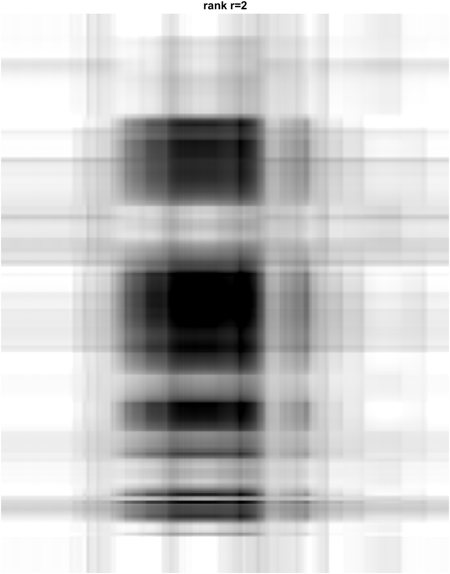
Here is the best rank 2 approximation for the image. Can you tell what the image is?
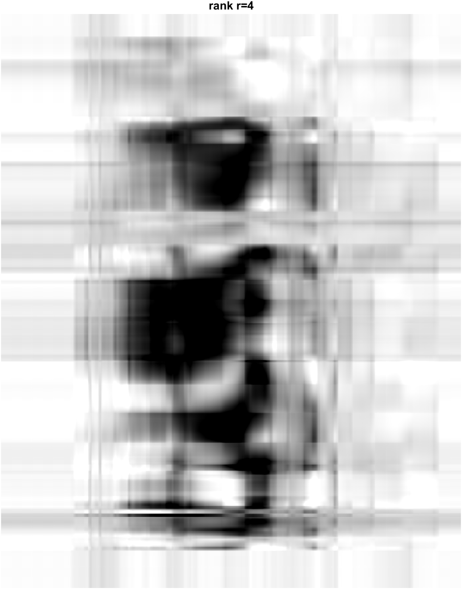
Here is the best rank 4 approximation for the image. Can you tell what the image is?
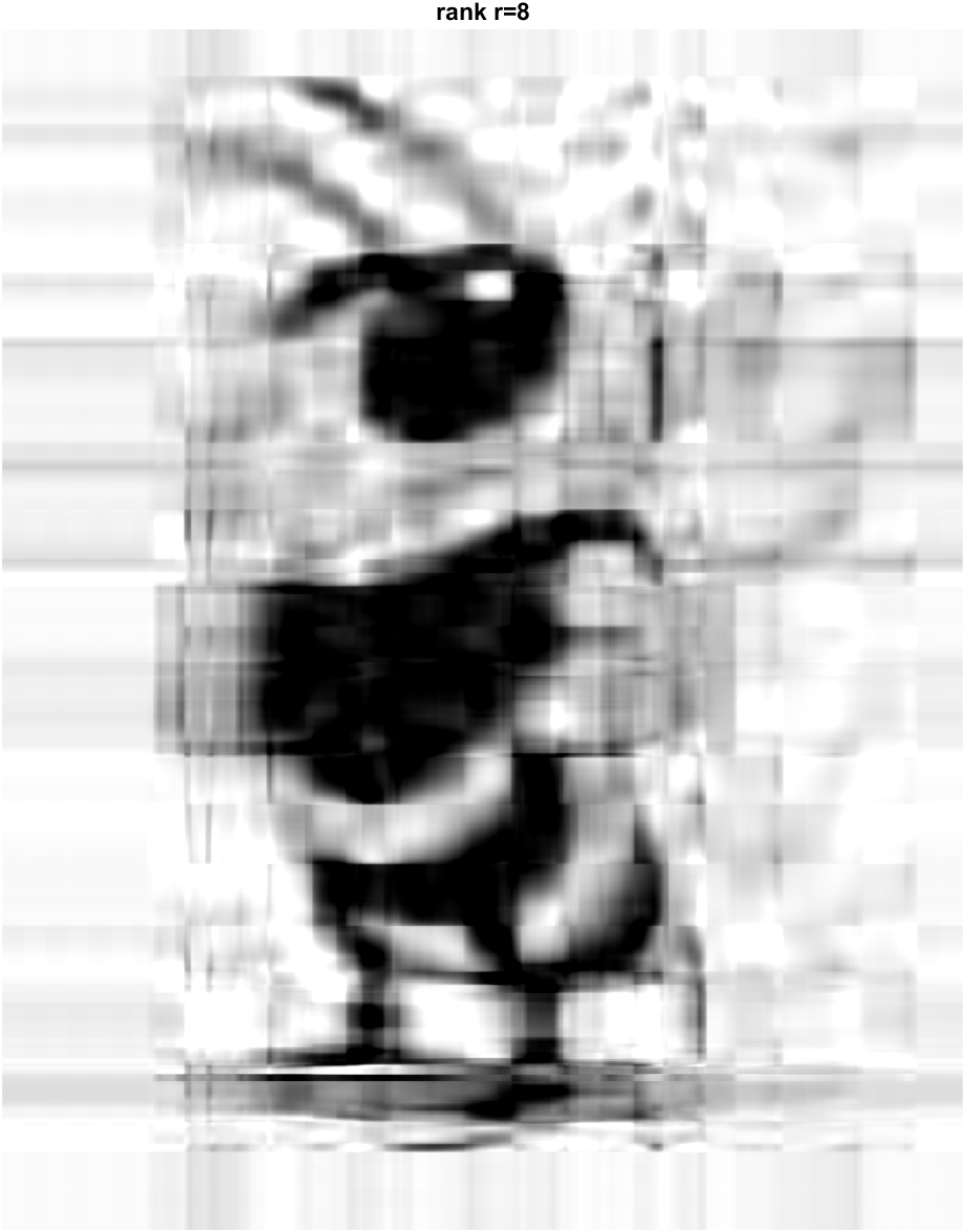
Here is the best rank 8 approximation for the image. Can you tell what the image is?
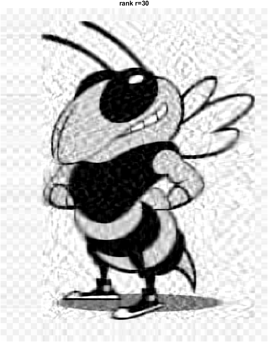
Here is the best rank 30 approximation for the image. Can you tell what the image is?