5.2 The Characteristic Equation

Print preview

Section 5.2 The Characteristic Equation

Handout 5.2 The Characteristic Equation

Objectives: Topics

The characteristic polynomial of a matrix

🔗
Algebraic and geometric multiplicity of eigenvalues

🔗

🔗

Objectives: Goals

Construct the characteristic polynomial of a matrix and use it to identify eigenvalues and their multiplicities.

🔗
Characterize the long-term behaviour of dynamical systems using eigenvalue decompositions.

🔗

🔗

Note 5.14.

Similar matrices are introduced in Section 5.2, but are not used until Section 5.3. We will wait to introduce them in Section 5.3.

🔗

Recall:

🔗

$\lambda$ is an eigenvalue of $A$ if and only if $(A-\lambda I)$ is not invertible.

🔗

Therefore, to calculate the eigenvalues of $A\text{,}$ we can need to find all $\lambda$ so that

🔗

\begin{equation*} \det(A-\lambda I)=0. \end{equation*}

Definition 5.15.

The quantity $\det(A-\lambda I)$ is the characteristic polynomial of $A\text{.}$

🔗

The equation $\det(A - \lambda I) = 0$ is the characteristic equation of $A\text{.}$

🔗

The roots of the characteristic polynomial are the eigenvalues of $A\text{.}$

🔗

Example 5.16.

Find the characteristic polynomial of

🔗

\begin{equation*} A=\begin{bmatrix} 5 \amp 2\\ 2 \amp 1 \end{bmatrix}. \end{equation*}

Then determine the eigenvalues of $A\text{.}$

🔗

Example 5.17.

Let

🔗

\begin{equation*} M=\begin{bmatrix} a \amp b\\ c \amp d \end{bmatrix}. \end{equation*}

Express the characteristic equation of $M$ in terms of $\det(M)\text{.}$ What is the equation when $M$ is singular?

🔗

Theorem 5.18.

Let $A$ be an $n \times n$ matrix with eigenvalues $\lambda_1, \dots, \lambda_n\text{.}$ Then, $\det(A) = \lambda_1\cdots\lambda_n$ and $\operatorname{tr}(A) = \lambda_1 + \cdots + \lambda_n\text{.}$

🔗

Definition 5.19. Algebraic Multiplicity.

The algebraic multiplicity of an eigenvalue is its multiplicity as a root of the characteristic polynomial.

🔗

Example 5.20.

Compute the algebraic multiplicities of the eigenvalues for

🔗

\begin{equation*} A = \begin{bmatrix} 1 \amp 0 \amp 0 \amp 0\\ 0 \amp 2 \amp 0 \amp 0\\ 0 \amp 0 \amp -1 \amp 1\\ 0 \amp 0 \amp 0 \amp -1 \end{bmatrix}. \end{equation*}

🔗

Definition 5.21. Geometric Multiplicity.

The geometric multiplicity of an eigenvalue $\lambda$ is the dimension of $\operatorname{Nul}(A-\lambda I)\text{.}$

🔗

The geometric multiplicity of an eigenvalue $\lambda$ is always between 1 and the algebraic multiplicity of $\lambda\text{.}$ It can never be 0 nor be greater than the algebraic mutliplicy.

🔗
Basic example:
\begin{equation*} \begin{bmatrix} 1 \amp 1\\ 0 \amp 1 \end{bmatrix} \end{equation*}
has only eigenvalue $\lambda=1\text{.}$ Its algebraic multiplicity is 2, but its geometric multiplicity is 1.

🔗

🔗

Example 5.22.

Compute the geometric multiplicities of the eigenvalues for

🔗

\begin{equation*} A = \begin{bmatrix} 1 \amp 0 \amp 0 \amp 0\\ 0 \amp 2 \amp 0 \amp 0\\ 0 \amp 0 \amp -1 \amp 1\\ 0 \amp 0 \amp 0 \amp -1 \end{bmatrix}. \end{equation*}

🔗

Example 5.23.

For each part below, give an example of a $5\times 5$ matrix withe the stated properties, if possible.

🔗

(a)

The only eigenvalue is $\lambda=0\text{,}$ but the geometric multiplicity of $\lambda=0$ is one.

🔗

(b)

The only eigenvalues are $\lambda_1=0$ and $\lambda_2 = 1\text{.}$ The algebraic multiplicity of $\lambda_1=0$ is three and the geometric multiplicity of $\lambda_2 = 1$ is three.

🔗

(c)

Exactly three eigenvalues, all with geometric multiplicity equal to 1.

🔗

Example 5.24.

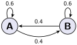
Consider the Markov Chain given by

🔗

\begin{equation*} \vec x_0= \begin{bmatrix} 1\\ 0 \end{bmatrix}, \quad \vec x_{k+1}=P\vec x_k = \begin{bmatrix} 0.6 \amp 0.4\\ 0.4 \amp 0.6 \end{bmatrix} \vec x_k. \end{equation*}