Skip to main content
Contents Embed Dark Mode Prev Up Next \(\newcommand{\foo}{b^{ar}}
\newcommand{\aug}{\fboxsep=-\fboxrule\!\!\!\fbox{\strut}\!\!\!}
\newcommand{\Nul}{\operatorname{Nul}}
\newcommand{\Col}{\operatorname{Col}}
\newcommand{\Row}{\operatorname{Row}}
\newcommand{\Span}{\operatorname{Span}}
\renewcommand{\det}{\operatorname{det}}
\newcommand{\rank}{\operatorname{rank}}
\newcommand{\proj}{\operatorname{proj}}
\newcommand{\dist}{\operatorname{dist}}
\newcommand{\lt}{<}
\newcommand{\gt}{>}
\newcommand{\amp}{&}
\definecolor{fillinmathshade}{gray}{0.9}
\newcommand{\fillinmath}[1]{\mathchoice{\colorbox{fillinmathshade}{$\displaystyle \phantom{\,#1\,}$}}{\colorbox{fillinmathshade}{$\textstyle \phantom{\,#1\,}$}}{\colorbox{fillinmathshade}{$\scriptstyle \phantom{\,#1\,}$}}{\colorbox{fillinmathshade}{$\scriptscriptstyle\phantom{\,#1\,}$}}}
\)
Section 1.8 An Introduction to Linear Transformations
Handout 1.8 An Introduction to Linear Transformations
Objectives: Topics
Objectives: Goals
Definition 1.49 .
Let
\(A\) be an
\(m\times n\) matrix. Define a function
\begin{equation*}
T:\mathbb{R}^n \to \mathbb{R}^m, \qquad T(\vec v) = A\vec v .
\end{equation*}
A function of this form is called a
matrix transformation .
The domain of \(T\) is \(\mathbb{R}^n\text{.}\)
The codomain (or target ) of \(T\) is \(\mathbb{R}^m\text{.}\)
The vector \(T(\vec x)\) is the image of \(\vec x\) under \(T\text{.}\)
The set of all possible images \(T(\vec x)\) is the range of \(T\text{.}\)
This yields another interpretation of the equation
\(A\vec x=\vec b\text{:}\)
Many familiar functions have domain and codomain
\(\mathbb{R}\text{.}\) For example, the sine function can be described by the rule
\begin{equation*}
f\colon \mathbb{R}\to\mathbb{R}, \qquad f(x)=\sin(x).
\end{equation*}
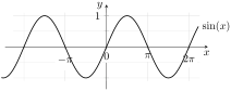
In calculus we often visualize a function via its graph: the horizontal axis represents the domain and the vertical axis the codomain.
Graph of \(y = \sin(x)\) on the interval \([-2\pi, 2\pi]\) with axes labeled \(x\) and \(y\) and a light grid.
Graphing is fine when both domain and codomain are
\(\mathbb{R}\text{.}\) If the domain is
\(\mathbb{R}^2\) and the codomain is
\(\mathbb{R}^3\text{,}\) we would need five dimensions to draw the full graph, so a geometric graph is not possible.
Example 1.50 .
Let
\(A=\begin{bmatrix} 1\amp 1\\[2pt] 0\amp 1\\[2pt] 1\amp 1 \end{bmatrix},\qquad
\vec u=\begin{bmatrix} 3\\[2pt] 4 \end{bmatrix},\qquad
\vec b=\begin{bmatrix} 7\\[2pt] 5\\[2pt] 7 \end{bmatrix}.\)
Consider the matrix transformation
\(T(\vec v)=A\vec v\text{.}\)
(a) Compute
\(T(\vec u)\text{.}\)
(b) Find
\(\vec v\in\mathbb{R}^2\) so that
\(T(\vec v)=\vec b\text{.}\)
(c) Give a vector
\(\vec c\in\mathbb{R}^3\) for which there is no
\(\vec v\) with
\(T(\vec v)=\vec c\text{.}\)
Equivalently: Give a
\(\vec c\) not in the range of
\(T\text{,}\) i.e., not in the span of the columns of
\(A\text{.}\)
Definition 1.51 .
A function \(T:\mathbb{R}^n\to\mathbb{R}^m\) is linear if for all \(\vec u,\vec v\in\mathbb{R}^n\) and all scalars \(c\in\mathbb{R}\text{:}\)
\(T(\vec u+\vec v)=T(\vec u)+T(\vec v)\text{,}\)
\(T(c\,\vec v)=c\,T(\vec v)\text{.}\)
By linearity, for any scalars \(c_1,\dots,c_k\) and vectors \(\vec v_1,\dots,\vec v_k\text{,}\)
\begin{equation*}
T\!\big(c_1\vec v_1+\cdots+c_k\vec v_k\big)
\;=\;
c_1\,T(\vec v_1)+\cdots+c_k\,T(\vec v_k).
\end{equation*}
This is the
principle of superposition . In particular, once we know
\(T(\vec e_1),\dots,T(\vec e_n)\text{,}\) we can compute
\(T(\vec v)\) for any
\(\vec v \in \mathbb{R}^n\text{.}\)
Fact 1.52 .
Every matrix transformation
\(T_A(\vec v)=A\vec v\) is linear.
Example 1.53 .
Suppose
\(T(\vec x)=A\vec x\text{.}\) Give a brief geometric description of the action of
\(T\) in
\(\mathbb{R}^2\) for each matrix.
(a)
\(A=\begin{bmatrix} 0\amp 1\\[2pt] 1\amp 0 \end{bmatrix}\)
(b)
\(A=\begin{bmatrix} 1\amp 0\\[2pt] 0\amp 0 \end{bmatrix}\)
(c)
\(A=\begin{bmatrix} k\amp 0\\[2pt] 0\amp k \end{bmatrix}\) for
\(k\in\mathbb{R}\)
Example 1.54 .
Describe the effect of
\(T_A\) on vectors in
\(\mathbb{R}^3\text{.}\)
(a)
\(A=\begin{bmatrix} 1\amp 0\amp 0\\[2pt] 0\amp 1\amp 0\\[2pt] 0\amp 0\amp 0 \end{bmatrix}\)
(b)
\(A=\begin{bmatrix} 1\amp 0\amp 0\\[2pt] 0\amp -1\amp 0\\[2pt] 0\amp 0\amp 1 \end{bmatrix}\)
Example 1.55 .
A linear transformation
\(T:\mathbb{R}^2\to\mathbb{R}^3\) satisfies
\begin{equation*}
T\!\left(\begin{bmatrix}1\\[2pt]0\end{bmatrix}\right)
=
\begin{bmatrix}5\\[2pt]-7\\[2pt]2\end{bmatrix},
\qquad
T\!\left(\begin{bmatrix}0\\[2pt]1\end{bmatrix}\right)
=
\begin{bmatrix}-3\\[2pt]8\\[2pt]0\end{bmatrix}.
\end{equation*}
What is the matrix that represents
\(T\text{?}\)