
Section 2.8 Subspaces

Handout 2.8 Subspaces

Motivating Question: Given a matrix \(A\text{,}\) what is the set of vectors \(\vec b\) for which we can solve \(A\vec x=\vec b\text{?}\)

Definition 2.35 Subset of \(\mathbb{R}^n\).

A subset of \(\mathbb{R}^n\) is any collection of vectors contained in \(\mathbb{R}^n\text{.}\)

Definition 2.36 Subspace.

A subset \(H\) of \(\mathbb{R}^n\) is a subspace if:
  • \(\displaystyle \vec 0 \in H\)
  • \(\vec u+\vec v\in H\) for all \(\vec u,\vec v\in H\text{.}\)
  • \(c\vec u\in H\) for any scalar \(c\in\mathbb{R}\) and any \(\vec u\in H\text{.}\)
Note that scalar closure implies the zero vector must be in \(H\text{.}\)

Example 2.37.

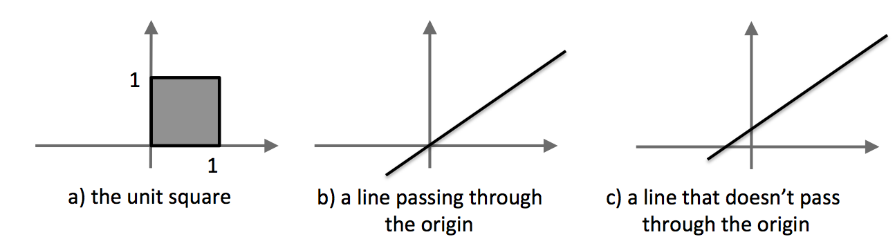
Which of the following subsets could be subspaces of \(\mathbb{R}^2\text{?}\)
A graphic showing three subsets of \(\mathbb{R}^2\text{.}\) The first (a) is the unit square. The second (b) is a line through the origin. The third (c) is a line that does not pass throught the origin.
Solution.
For (a), note that the unit square contains the vector \(\vec v = \begin{bmatrix} 1 \\ 1 \end{bmatrix}\text{,}\) but does not contain the vector \(2\vec v = \begin{bmatrix} 2 \\ 2 \end{bmatrix}\text{.}\) Therefore, the unit square is NOT a subspace of \(\mathbb{R}^2\text{.}\)
For (b), first note that the line passes throught the origin, so the subset contains \(\vec 0\text{.}\) Next, if \(\vec v\) is a nonzero vector on the line, we see that every vector on the line can be expressed as some multiple of \(\vec v\text{.}\) Therefore, the subset can be written as \(\left\{t\vec v \ \rvert \ t\in\mathbb{R}\right\} = \operatorname{Span}\left\{\vec v\right\}\text{.}\) It follows that the subset is closed under vector addition and scalar multiplication. Hence, a line passing throught the origin IS as subpace of \(\mathbb{R}^2\text{.}\)
For (c), note that the line does NOT pass through the origin. So the subset does NOT contain \(\vec 0\) and is NOT a subspace of \(\mathbb{R}^2\text{.}\)

Example 2.38.

For each subset of \(\mathbb{R}^3\) given below, determine if it is a subspace of \(\mathbb{R}^3\text{.}\)

(a)

\(S_1 = \left\{\vec 0\right\}\)
Solution.
Note that \(\vec 0 \in S_1\text{.}\) Also, we have that \(S_1\) is closed under vector addition and scalar multiplication since every vector you choose in \(S_1\) has to be \(\vec 0\) since it is the only vector in \(S_1\text{.}\) Thus, \(S_1\) is a subspace of \(\mathbb{R}^3\text{.}\)

(b)

\(S_2 = \left\{\vec 0, \begin{bmatrix} 1 \\ 0 \\ 1 \end{bmatrix},\begin{bmatrix}-1 \\ 0 \\ -1\end{bmatrix} \right\}\)
Solution.
Note that \(\begin{bmatrix} 1 \\ 0 \\ 1 \end{bmatrix} \in S_2\text{,}\) but \(2\begin{bmatrix}1 \\ 0 \\ 1 \end{bmatrix} = \begin{bmatrix} 2 \\ 0 \\ 2 \end{bmatrix} \not \in S_2\text{.}\) Therefore, \(S_2\) is NOT closed under scalar multiplication, so \(S_2\) is NOT a subspace of \(\mathbb{R}^3\text{.}\)

(c)

\(S_3 = \left\{\begin{bmatrix}1 \\ 0 \\ 0 \end{bmatrix}, \begin{bmatrix} 0 \\ 1 \\ 0 \end{bmatrix}, \begin{bmatrix} 0 \\ 0 \\ 1 \end{bmatrix}\right\}\)
Solution.
Note that \(\begin{bmatrix} 1 \\ 0 \\ 0 \end{bmatrix}, \begin{bmatrix} 0 \\ 1 \\ 0 \end{bmatrix} \in S_3\text{,}\) but \(\begin{bmatrix} 1 \\ 0 \\ 0 \end{bmatrix} + \begin{bmatrix} 0 \\ 1 \\ 0 \end{bmatrix} = \begin{bmatrix} 1 \\ 1 \\ 0 \end{bmatrix} \not \in S_3\text{.}\) Thus, \(S_3\) is not closed under vector addition, so \(S_3\) is NOT a subspace of \(\mathbb{R}^3\text{.}\)

(d)

\(S_4 = \operatorname{Span}\left\{\begin{bmatrix}1 \\ 0 \\ 0 \end{bmatrix}, \begin{bmatrix} 0 \\ 1 \\ 0 \end{bmatrix}, \begin{bmatrix} 0 \\ 0 \\ 1 \end{bmatrix}\right\}\)
Solution.
Since \(S_4\) is the span of a set of vectors, we know that \(S_4\) contains every possible linear combination of its vectors. Therefore, \(S_4\) must contain \(\vec 0\) and must be closed under vector addition and scalar multiplication. Hence, \(S_4\) is a subspace of \(\mathbb{R}^3\text{.}\)

Example 2.39.

The following subsets of \(\mathbb{R}^2\) are written in set-builder notation. For each, determine if it is a subspace of \(\mathbb{R}^2\text{.}\) Note that \(\mathbb{Z} = \{\dots, -2, -1, 0, 1 , 2, \dots\}\) is the set of integers.

(a)

\(T_1 = \left\{\begin{bmatrix} x \\ -x \end{bmatrix} \in \mathbb{R}^2 \ \Big \rvert \ x\in\mathbb{Z}\right\}\)
Solution.
Note that \(\begin{bmatrix} 1 \\ -1 \end{bmatrix} \in T_1\text{,}\) but \(\pi\begin{bmatrix}1 \\ -1 \end{bmatrix} = \begin{bmatrix} \pi \\ -\pi \end{bmatrix} \not \in T_1\) since \(\pi\) is not an integer. Therefore, \(T_1\) is NOT closed under scalar multiplication, so \(T_1\) is NOT a subspace of \(\mathbb{R}^2\text{.}\)

(b)

\(T_2 = \left\{\begin{bmatrix} x \\ -x \end{bmatrix} \in \mathbb{R}^2 \ \Big \rvert \ x\in\mathbb{R}\right\}\)
Solution.
Note that \(T_2 = \operatorname{Span}\left\{\begin{bmatrix} 1 \\ -1 \end{bmatrix}\right\}\text{.}\) It follows that \(T_2\) is a subspace of \(\mathbb{R}^2\text{.}\)

(c)

\(T_3 = \left\{\vec x \in \mathbb{R}^2 \ \Big \rvert \ \begin{bmatrix} 1 \amp 2 \\ 2 \amp 4 \end{bmatrix}\vec x = \begin{bmatrix} 0 \\ 0 \end{bmatrix}\right\}\)
Solution.
Note that \(T_3 = \operatorname{Span}\left\{\begin{bmatrix} 2 \\ -1 \end{bmatrix}\right\}\text{.}\) It follows that \(T_3\) is a subspace of \(\mathbb{R}^2\text{.}\) In fact, the solution set of any homogeneous system is a subspace of \(\mathbb{R}^n\text{.}\) This subspace is called the nullspace (see DefinitionΒ 2.41).

(d)

\(T_4 = \left\{\vec x \in \mathbb{R}^2 \ \Big \rvert \ \begin{bmatrix} 1 \amp 2 \\ 2 \amp 4 \end{bmatrix}\vec x = \begin{bmatrix} 1 \\ 2 \end{bmatrix}\right\}\)
Solution.
Note that \(\vec 0 \not \in T_4\text{,}\) so \(T_4\) is NOT a subspace of \(\mathbb{R}^2\text{.}\) In fact, the solution set of any inhomogeneous system is NOT a subspace of \(\mathbb{R}^n\text{.}\)
Recall that for vectors \(\vec v_1,\dots,\vec v_p\in\mathbb{R}^n\text{,}\) \(\operatorname{Span}\{\vec v_1,\dots,\vec v_p\}\) is the subspace consisting of all linear combinations of these vectors. Not only is the span of vectors an example of a subspace of \(\mathbb{R}^n\text{,}\) they are the only examples of subspace of \(\mathbb{R}^n\text{.}\)

Definition 2.41 Column Space and Null Space.

Let \(A=\begin{bmatrix}\vec a_1 \amp \cdots \amp \vec a_n\end{bmatrix}\) be an \(m\times n\) matrix.
  • The column space of \(A\text{,}\) \(\operatorname{Col}(A)\text{,}\) is the subspace of \(\mathbb{R}^m\) spanned by \(\vec a_1,\dots,\vec a_n\text{.}\)
  • The null space of \(A\text{,}\) \(\operatorname{Nul}(A)\text{,}\) is the subspace of \(\mathbb{R}^n\) consisting of all solutions to \(A\vec x=\vec 0\text{.}\)

Example 2.43.

Is \(\vec b\) in the column space of \(A\text{?}\)
\begin{equation*} A= \begin{bmatrix} 1 \amp -3 \amp -4\\ -4 \amp 6 \amp -2\\ -3 \amp 7 \amp 6 \end{bmatrix} \sim \begin{bmatrix} 1 \amp 0 \amp 5\\ 0 \amp 1 \amp 3\\ 0 \amp 0 \amp 0 \end{bmatrix} = B, \qquad \vec b= \begin{bmatrix} 3\\3\\-4 \end{bmatrix}. \end{equation*}
Solution.
By TheoremΒ 1.37, asking whether \(\vec b \in \operatorname{Col}(A)\) is equivalent to asking whether the matrix equation \(A\vec x = \vec b\) has a solution. By TheoremΒ 2.42, we must augment with the matrix \(A \) and cannot augment with \(B\text{.}\) Note that
\begin{equation*} \begin{bmatrix} A \amp \rvert \amp \vec b \end{bmatrix} = \begin{bmatrix} 1 \amp -3 \amp -4 \amp \rvert \amp 3 \\ -4 \amp 6 \amp -2 \amp \rvert \amp 3 \\ -3 \amp 7 \amp 6 \amp \rvert \amp -4 \end{bmatrix} \sim \cdots \sim \begin{bmatrix} 1 \amp -3 \amp 4 \amp \rvert \amp 3 \\ 0 \amp 2 \amp 6 \amp \rvert \amp -5 \\ 0 \amp 0 \amp 0 \amp \rvert \amp 0 \end{bmatrix}\text{.} \end{equation*}
Since we do not have a pivot in the augmented column, the system \(A\vec x = \vec b\) is consistent. Hence, \(\vec b \in \operatorname{Col}(A)\text{.}\)
You can find a particular linear combination of the columns of \(A\) which produce \(\vec b\) by continuing to solve the system.

Example 2.44.

Determine whether \(\vec v\) is in \(\operatorname{Nul}(A)\text{.}\)
\begin{equation*} A = \begin{bmatrix} 1 \amp -3 \amp -4\\ -4 \amp 6 \amp -2\\ -3 \amp 7 \amp 6 \end{bmatrix} \sim \begin{bmatrix} 1 \amp 0 \amp 5\\ 0 \amp 1 \amp 3\\ 0 \amp 0 \amp 0 \end{bmatrix} = B, \qquad \vec v= \begin{bmatrix} -5t\\ -3t\\ t \end{bmatrix}, \quad t\in\mathbb{R}. \end{equation*}
Solution.
By TheoremΒ 2.42, we are free to check whether \(A\vec v = \vec 0\) or \(B\vec v = \vec 0\) since \(\operatorname{Nul}(A) = \operatorname{Nul}(B)\text{.}\) Note that
\begin{equation*} A\vec v = \begin{bmatrix} 1 \amp -3 \amp -4 \\ -4 \amp 6 \amp -2\\ -3 \amp 7 \amp 6 \end{bmatrix} \begin{bmatrix} -5t \\ -3t \\ t \end{bmatrix} = \begin{bmatrix} -5t + 9t - 4t \\ 20t - 18t - 2t \\ 15t - 21t + 6t \end{bmatrix} = \begin{bmatrix} 0 \\ 0 \\ 0 \end{bmatrix}\text{.} \end{equation*}
Thus, \(\vec v \in \operatorname{Nul}(A)\) for any value of \(t\text{.}\)
Let’s determine if there are any other vectors in \(\Nul(A)\text{.}\) Since \(\Nul(A) = \Nul(B),\) we determine all solutions to \(B\vec x = \vec 0\text{.}\) Since \(B\) is already in RREF, we see that \(x_3 = t \in \mathbb{R}\) is a free variable and \(x_2 = -3t\) and \(x_1 = -5t\) are pivot variables. It follows that
\begin{equation*} \Nul(A) = \Nul(B) = \left\{\begin{bmatrix} -5t \\ 3t \\ t \end{bmatrix} \ \Big \rvert \ t \in \mathbb{R}\right\} = \Span\left\{\begin{bmatrix} -5 \\ -2 \\ 1 \end{bmatrix}\right\}. \end{equation*}

Definition 2.45 Basis.

A basis for a subspace \(H\) is a set of linearly independent vectors in \(H\) that span \(H\text{.}\)
In MATH 1554, each basis will be a finite set of vectors. For every subspace other than the trivial subspace \(\left\{\vec 0\right\}\text{,}\) there are infinitely many choices for the basis.
Be careful to NEVER include \(\Span\) when writing your basis. Writing \(\Span\) of the basis gives the entire subspace. A basis is NOT the entire subspace, but a finite set of building blocks used to build the space.

Example 2.46.

\begin{equation*} H=\left\{ \begin{bmatrix} x_1\\x_2\\x_3\\x_4 \end{bmatrix} \in\mathbb{R}^4\;\middle|\; x_1+2x_2+x_3+5x_4=0 \right\}. \end{equation*}

(a)

Find at least three vectors which live in \(H\text{.}\)
Solution.
We have the following
  • \(\vec 0 = \begin{bmatrix} 0 \\ 0 \\ 0 \\ 0 \end{bmatrix} \in H\) since \(0 + 2(0) + 0 + 5(0) = 0.\)
  • \(\begin{bmatrix} 2 \\ -1 \\ 5 \\ -1 \end{bmatrix} \in H\) since \(2 + 2(-1) + 5 + 5(-1) = 0.\)
  • \(\begin{bmatrix} 1 \\ 0 \\ -1 \\ 0 \end{bmatrix} \in H\) since \(1 + 2(0) + -1 + 5(0) = 0.\)

(b)

Find a matrix \(A\) such that \(H=\operatorname{Nul}(A)\text{.}\)
Solution.
Note that if \(A = \begin{bmatrix} 1 \amp 2 \amp 1 \amp 5 \end{bmatrix} \text{,}\) then
\begin{equation*} A\vec x = \vec 0 \implies \begin{bmatrix} 1 \amp 2 \amp 1 \amp 5 \end{bmatrix}\begin{bmatrix} x_1 \\ x_2 \\ x_3 \\ x_4 \end{bmatrix} = \vec 0 \implies \begin{bmatrix}x_1 + 2x_2 + x_3 + 5x_4\end{bmatrix} = \begin{bmatrix} 0 \end{bmatrix}\text{,} \end{equation*}
which is the defining characteristic of the vectors in \(H\text{.}\) Therefore, \(H = \Nul(A)\text{.}\)

(c)

Construct a basis for \(H\text{.}\)
Solution.
Note that the second, third, and fourth columns of \(A \) correspond to free variables. Therefore, \(x_4 = t \in \mathbb{R}, x_3 = r \in \mathbb{R},\) and \(x_2 = p\in\mathbb{R}\) are the free variables and \(x_1 = -2p - r - 5t\) is the pivot variables. It follows that
\(\begin{eqnarray*} \Nul(A) \amp = \amp \left\{\begin{bmatrix} -2p - r - 5t \\ p \\ r \\ t \end{bmatrix} \ \Big \rvert \ p,r,t\in\mathbb{R}\right\}\\ \amp = \amp \left\{p\begin{bmatrix}-2 \\ 1 \\ 0 \\ 0 \end{bmatrix} + r\begin{bmatrix} -1 \\ 0 \\ 1 \\ 0 \end{bmatrix} + t \begin{bmatrix} -5 \\ 0 \\ 0 \\ 1\end{bmatrix} \ \Big \rvert \ p,r,t\in\mathbb{R}\right\}\\ \amp = \amp \Span\left\{\begin{bmatrix} -2 \\ 1 \\ 0 \\ 0 \end{bmatrix}, \begin{bmatrix} -1 \\ 0 \\ 1 \\ 0 \end{bmatrix}, \begin{bmatrix} -5 \\ 0 \\ 0 \\ 1 \end{bmatrix}\right\}\end{eqnarray*}\)
Therefore, we see that the three vectors \(\begin{bmatrix} -2 \\ 1 \\ 0 \\ 0 \end{bmatrix}, \begin{bmatrix} -1 \\ 0 \\ 1 \\ 0 \end{bmatrix}, \begin{bmatrix} -5 \\ 0 \\ 0 \\ 1 \end{bmatrix}\) span \(\Nul(A)\text{.}\) Since they are linearly independent, they form a basis for \(\Nul(A)\text{.}\) Thus, a basis for \(\Nul(A)\) is the set of vectors
\begin{equation*} \left\{\begin{bmatrix} -2 \\ 1 \\ 0 \\ 0 \end{bmatrix}, \begin{bmatrix} -1 \\ 0 \\ 1 \\ 0 \end{bmatrix}, \begin{bmatrix} -5 \\ 0 \\ 0 \\ 1 \end{bmatrix}\right\}\text{.} \end{equation*}
This basis is NOT unique. Note you can replace any of the three vectors with a nonzero multiple of itself. Also, you could replace one of them with suitable linear combination. For example, you could replace the middle vector with the first place the second and that would still yield a valid basis since the resulting three vectors would be linearly independent and span the space.

Example 2.47.

Construct a basis for \(\operatorname{Nul}(A)\) and \(\operatorname{Col}(A)\text{.}\)
\begin{equation*} A= \begin{bmatrix} -3 \amp 6 \amp -1 \amp 0\\ 1 \amp -2 \amp 2 \amp 0\\ 2 \amp -4 \amp 5 \amp 0 \end{bmatrix} \sim \begin{bmatrix} 1 \amp -2 \amp 0 \amp 0\\ 0 \amp 0 \amp 1 \amp 0\\ 0 \amp 0 \amp 0 \amp 0 \end{bmatrix} = B. \end{equation*}
Solution.
First, note that we can express \(\Nul(A)\) as the span of some vectors by finding all solutions to \(A\vec x = \vec 0\text{.}\) It follows that
\begin{equation*} \Nul(A) = \Nul(B) = \Span\left\{\begin{bmatrix} 2 \\ 1 \\ 0 \\ 0 \end{bmatrix}, \begin{bmatrix} 0 \\ 0 \\ 0 \\ 1 \end{bmatrix}\right\}. \end{equation*}
Thus, a basis for \(\Nul(A)\) is
\begin{equation*} \mathcal{B} = \left\{\begin{bmatrix} 2 \\ 1 \\ 0 \\ 0 \end{bmatrix}, \begin{bmatrix} 0 \\ 0 \\ 0 \\ 1 \end{bmatrix}\right\}. \end{equation*}
By the definition of \(\Col(A)\text{,}\) we see that
\begin{equation*} \Col(A) = \Span\left\{\begin{bmatrix} -3 \\ 1 \\ 2 \end{bmatrix}, \begin{bmatrix} 6 \\ -2 \\ -4 \end{bmatrix}, \begin{bmatrix} -1 \\ 2 \\ 5 \end{bmatrix}, \begin{bmatrix} 0 \\ 0 \\ 0 \end{bmatrix}\right\}. \end{equation*}
Note that the set containing the four column vectors of \(A \) is NOT a basis since those vectors are NOT linearly independent. From \(B\text{,}\) we see that Column 2 and Column 4 of \(A\) are NOT pivot columns. Therefore, they are linearly dependent on the other columns of \(A\text{.}\) It follows that the following set containing Column 1 and Column 2 of \(A\) spans \(\Col(A)\) and is linearly independent, so it is a basis for \(\Col(A)\text{.}\)
\begin{equation*} \mathcal{C} = \left\{\begin{bmatrix} -3 \\ 1 \\ 2 \end{bmatrix}, \begin{bmatrix} -1 \\ 2 \\ 5 \end{bmatrix}\right\} \end{equation*}
Example 2.48.

\begin{equation*} V=\left\{ \begin{bmatrix} a\\b \end{bmatrix} \in\mathbb{R}^2\;\middle|\;ab=0 \right\}. \end{equation*}

(a)

Give an example of a vector that is in \(V\text{.}\)
Solution.
Note that \(\begin{bmatrix} 1 \\ 0 \end{bmatrix} \in V\) since \(1(0) = 0\) and \(\begin{bmatrix} 0 \\ 1 \end{bmatrix} \in V\) since \(0(1) = 0\text{.}\)

(b)

Give an example of a vector that is not in \(V\text{.}\)
Solution.
Note that \(\begin{bmatrix} 1 \\ 1 \end{bmatrix} \not \in V\) since \(1(1) = 1 \neq 0.\)

(c)

Is the zero vector in \(V\text{?}\)
Solution.
Yes, \(\vec 0 = \begin{bmatrix} 0 \\ 0 \end{bmatrix} \in V\) since \(0(0) = 0\text{.}\)

(d)

Is \(V\) a subspace of \(\mathbb{R}^2\text{?}\)
Solution.
From (a) and (b), we see that \(\begin{bmatrix} 1 \\ 0 \end{bmatrix}, \begin{bmatrix} 0 \\ 1 \end{bmatrix} \in V\text{,}\) but \(\begin{bmatrix} 1 \\ 0 \end{bmatrix} + \begin{bmatrix} 0 \\ 1 \end{bmatrix} = \begin{bmatrix} 1 \\ 1 \end{bmatrix} \not \in V\text{.}\) Thus, \(V \) is not closed under vector addition. Hence, \(V \) is NOT a subspace of \(\mathbb{R}^2\text{.}\)