Objectives: Topics
Objectives: Goals
Apply least-squares and mutiple regression to construct a linear model from a set of data points.
Apply least-squares to fit polynomials and other curves to data.
One of the most useful applications of finding least squares solutions is to determine curves of best fit for data.
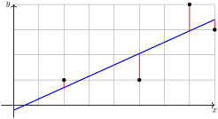
The graph above gives an approximate linear relationship between \(x\) and \(y\text{.}\)
The black circles are data.
The blue line is the
least squares line , also known as the
line of best fit .
The lengths of the red lines are the
errors between our line of best fit and the data.
The
least squares line minimizes the sum of squares of the errors.
We can use this technique to find line of best fit even when there are more than two variables.
Example 6.61 .
Suppose we are trying to predict house prices based on two factors:
\(x_1 = \) size (in 1000 sq ft)
\(x_2 = \) number of bedrooms
We have the following data:
Table 6.62. Housing Data
Size (in 1000 sq ft)
Number of Bedrooms
Price (in $1000s)
1.0
1
180
2.0
2
260
3.0
3
310
4.0
3
350
(a)
Setup the least-squares problem which will produce the best linear model for this situation:
\begin{equation*}
y = \beta_0 + \beta_1 x_1 + \beta_2 x_2\text{.}
\end{equation*}
(b)
Solving the system above, we find that
\begin{equation*}
\widehat \beta = \begin{bmatrix} \beta_0 \\ \beta_1 \\ \beta_2 \end{bmatrix} = \begin{bmatrix} 120 \\ 35 \\ 30\end{bmatrix}\text{.}
\end{equation*}
According to this model, how much should a house with 2000 ft\(^2\) and 3 bedrooms be worth?
We do not have to restrict ourselves to linear curves of best fit. All that is required to use Least Squares is that the unknowns we are trying to solve for, our coefficients, are linear. There is nothing wrong with allowing the variables to be nonlinear.
In general, we can consider least squares fitting for the form
\begin{equation*}
y = \beta_0 + \beta_1 f_1(x_1, \dots, x_m) + \beta_2 f_2(x_1, \dots, x_m) + \cdots + \beta_n f_n(x_1, \dots, x_m)\text{,}
\end{equation*}
where the functions \(f_i\) are known, but not necessarily linear. Keep in mind that this is a linear problem in the \(\beta_i\) variables.
Example 6.63 .
For the remaining four examples, we will fit various curves to the following points:
\begin{equation*}
(-1,-3), (0,0), (1,3), (2,2)\text{.}
\end{equation*}
Once you find the curve, graph the points and the curve on Desmos and see how good the curve fits.
We will start by fitting a linear curve to the data:
\begin{equation*}
y = \beta_0 + \beta_1 x\text{.}
\end{equation*}
This one can be solved without the need of a calculator.