Suppose we wish to find the maximum and minimum values of
\begin{equation*}
Q(\vec x)=\vec x^{\,T}A\vec x
\end{equation*}
subject to the constraint
\(\|\vec x\|=1\text{.}\)
\begin{equation*}
m=\min\{Q(\vec x)\mid \|\vec x\|=1\},\qquad
M=\max\{Q(\vec x)\mid \|\vec x\|=1\}.
\end{equation*}
This is an example of a
constrained optimization problem. We are also interested in where these extreme values are attained.
These problems are straight-forward when
\(Q(\vec x)\) has no cross-product terms. What about when it does have cross-product terms?
Example 7.32.
Calculate the maximum and minimum values of
\begin{equation*}
Q(\vec x)=x_2^2 + 2x_1x_3.
\end{equation*}
where
\(\vec x\in\mathbb{R}^3\) and
\(\|\vec x\|=1\text{.}\) Identify the points where these values are obtained.
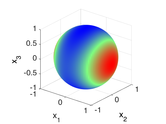
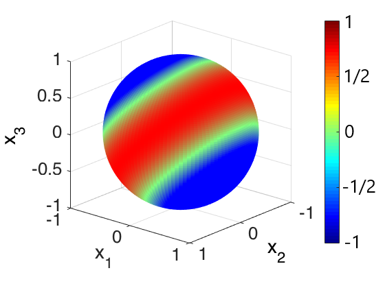
The image below is the unit sphere whose surface is colored according to the quadratic form from
Example 7.32. Notice the agreement between our solution and the image.
Theorem 7.33. Extrema via Eigenvalues.
Let
\(Q(\vec x)=\vec x^{\,T}A\vec x\text{,}\) where
\(A\) is a real symmetric
\(n\times n\) matrix with eigenvalues
\begin{equation*}
\lambda_1 \ge \lambda_2 \ge \cdots \ge \lambda_n
\end{equation*}
and corresponding
normalized eigenvectors
\begin{equation*}
\vec u_1,\vec u_2,\ldots,\vec u_n.
\end{equation*}
Under the constraint
\(\|\vec x\|=1\text{:}\)
-
The maximum value of \(Q\) is \(\lambda_1\text{,}\) attained at \(\vec x=\pm\vec u_1\text{.}\)
-
The minimum value of \(Q\) is \(\lambda_n\text{,}\) attained at \(\vec x=\pm\vec u_n\text{.}\)
Example 7.34.
Calculate the maximum value of
\(Q(\vec x)=\vec x^{\,T}A\vec x\text{,}\) with
\(\vec x\in\mathbb{R}^3\text{,}\) subject to the constraint
\(\|\vec x\|=5\text{.}\) Identify a point where this maximum is obtained.
\begin{equation*}
Q(\vec x)=x_2^2 + 2x_1x_3.
\end{equation*}
Theorem 7.35. Extrema with an Orthogonality Condition.
Let
\(Q(\vec x)=\vec x^{\,T}A\vec x\text{,}\) where
\(A\) is a real symmetric
\(n\times n\) matrix with eigenvalues
\begin{equation*}
\lambda_1 \ge \lambda_2 \ge \cdots \ge \lambda_n
\end{equation*}
and corresponding eigenvectors
\begin{equation*}
\vec u_1,\vec u_2,\ldots,\vec u_n.
\end{equation*}
Subject to the constraints
\(\|\vec x\|=1\) and
\(\vec x\cdot\vec u_1=0\text{:}\)
-
The maximum value of \(Q\) is \(\lambda_2\text{,}\) attained at an eigenvector associated to \(\lambda_2\text{.}\)
-
The minimum value of \(Q\) is \(\lambda_n\text{,}\) attained at \(\vec u_n\text{.}\)
Here
\(\lambda_2\) denotes the
second largest eigenvalue of
\(A\text{.}\)
Example 7.36.
Calculate the maximum and minimum values of
\begin{equation*}
Q(\vec x)=\vec x^T A \vec x = x_1^2 + x_2^2 + x_3^2 + 6x_1x_2\text{,}
\end{equation*}
with \(\vec x\in\mathbb{R}^3\text{,}\) subject to \(\|\vec x\|=1\) and \(\vec x\cdot\vec u_1=0\text{,}\) where
\begin{equation*}
A = \begin{bmatrix} 1 \amp 3 \amp 0 \\ 3 \amp 1 \amp 0 \\ 0 \amp 0 \amp 1 \end{bmatrix} \quad \text{and} \quad \vec u_1=\begin{bmatrix}1\\1\\0\end{bmatrix}\text{.}
\end{equation*}
Identifu points where the maximum and minimum values occur. The eigenvalues of \(A\) are \(\lambda = 4, 1, -2\text{.}\)