Skip to main content
Contents Embed Dark Mode Prev Up Next \(\newcommand{\foo}{b^{ar}}
\newcommand{\aug}{\fboxsep=-\fboxrule\!\!\!\fbox{\strut}\!\!\!}
\newcommand{\Nul}{\operatorname{Nul}}
\newcommand{\Col}{\operatorname{Col}}
\newcommand{\Row}{\operatorname{Row}}
\newcommand{\Span}{\operatorname{Span}}
\renewcommand{\det}{\operatorname{det}}
\newcommand{\rank}{\operatorname{rank}}
\newcommand{\proj}{\operatorname{proj}}
\newcommand{\dist}{\operatorname{dist}}
\newcommand{\lt}{<}
\newcommand{\gt}{>}
\newcommand{\amp}{&}
\definecolor{fillinmathshade}{gray}{0.9}
\newcommand{\fillinmath}[1]{\mathchoice{\colorbox{fillinmathshade}{$\displaystyle \phantom{\,#1\,}$}}{\colorbox{fillinmathshade}{$\textstyle \phantom{\,#1\,}$}}{\colorbox{fillinmathshade}{$\scriptstyle \phantom{\,#1\,}$}}{\colorbox{fillinmathshade}{$\scriptscriptstyle\phantom{\,#1\,}$}}}
\)
Section 6.5 Least-Squares Problems
Handout 6.5 Least-Squares Problems
Objectives: Topics
Objectives: Goals
Compute general solutions and least squares errors using both:
the normal equations
the QR decomposition
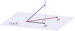
Definition 6.50 . Least Squares Solution.
Let
\(A\) be an
\(m\times n\) matrix. A vector
\(\widehat x\) is a
least squares solution to
\(A\vec x=\vec b\) if
\begin{equation*}
\lVert\vec b - A\widehat x\rVert
\le
\lVert\vec b - A\vec x\rVert
\quad \text{for all } \vec x\in\mathbb{R}^n.
\end{equation*}
Example 6.52 .
Consider the system \(A\vec x = \vec b\) for
\begin{equation*}
A = \begin{bmatrix} 4 \amp 0 \\ 0 \amp 2 \\ 1 \amp 1 \end{bmatrix} \quad \text{and} \quad \vec b = \begin{bmatrix} 2 \\ 0 \\ 11 \end{bmatrix}\text{.}
\end{equation*}
(a) Is the system consistent?
(b) Find the vector
\(\widehat b = \proj_{\Col(A)}\vec b\text{.}\)
(c) Find the
least squares solution to
\(A\vec x = \vec b\text{.}\)
Theorem 6.54 . Normal Equations for Least Squares.
Least squares solutions of
\(A\vec x=\vec b\) are precisely the solutions of
\begin{equation*}
A^T A\vec x = A^T\vec b,
\end{equation*}
refered to as the
normal equations .
Example 6.55 .
Use the normal equations to find the least-squares solution of
\(A\vec x=\vec b\text{,}\) where
\begin{equation*}
A=\begin{bmatrix}
4 \amp 0\\
0 \amp 2\\
1 \amp 1
\end{bmatrix},
\qquad
\vec b=\begin{bmatrix}
2\\0\\11
\end{bmatrix}.
\end{equation*}
Theorem 6.56 . Unique Least Squares Solutions.
For an
\(m\times n\) matrix
\(A\text{,}\) the following are equivalent:
For every \(\vec b\text{,}\) the equation \(A\vec x=\vec b\) has a unique least squares solution.
The columns of \(A\) are linearly independent.
\(A^TA\) is invertible.
\begin{equation*}
\widehat x = (A^TA)^{-1}A^T\vec b.
\end{equation*}
Example 6.57 .
Compute the least squares solution to
\(A\vec x = \vec b\text{,}\) where
\begin{equation*}
A=\begin{bmatrix}
1 \amp -6\\
1 \amp -2\\
1 \amp 1\\
1 \amp 7
\end{bmatrix},
\qquad
\vec b=\begin{bmatrix}
-1\\2\\1\\6
\end{bmatrix}.
\end{equation*}
Theorem 6.58 . Least Squares via QR Factorization.
If
\(A=QR\) is a QR decomposition of an
\(m\times n\) matrix
\(A\text{,}\) then for any
\(\vec b\) the least squares solution of
\(A\vec x=\vec b\) satisfies:
\begin{equation*}
R\widehat x = Q^T\vec b.
\end{equation*}
Example 6.59 .
Compute the least squares solution to
\(A\vec x=\vec b\text{,}\) where
\begin{equation*}
A=
\begin{bmatrix}
1 \amp 3 \amp 5\\
1 \amp 1 \amp 0\\
1 \amp 1 \amp 2\\
1 \amp 3 \amp 3
\end{bmatrix},
\qquad
\vec b=\begin{bmatrix}
3\\5\\7\\-3
\end{bmatrix}
\end{equation*}
given the QR factorization:
\begin{equation*}
A = \dfrac{1}{2}
\begin{bmatrix}
1 \amp 1 \amp 1\\
1 \amp -1 \amp -1\\
1 \amp -1 \amp 1\\
1 \amp 1 \amp -1
\end{bmatrix}
\begin{bmatrix}
2 \amp 4 \amp 5\\
0 \amp 2 \amp 3\\
0 \amp 0 \amp 2
\end{bmatrix}.
\end{equation*}