Skip to main content\(\newcommand{\foo}{b^{ar}}
\newcommand{\aug}{\fboxsep=-\fboxrule\!\!\!\fbox{\strut}\!\!\!}
\newcommand{\Nul}{\operatorname{Nul}}
\newcommand{\Col}{\operatorname{Col}}
\newcommand{\Row}{\operatorname{Row}}
\newcommand{\Span}{\operatorname{Span}}
\renewcommand{\det}{\operatorname{det}}
\newcommand{\rank}{\operatorname{rank}}
\newcommand{\proj}{\operatorname{proj}}
\newcommand{\dist}{\operatorname{dist}}
\newcommand{\lt}{<}
\newcommand{\gt}{>}
\newcommand{\amp}{&}
\definecolor{fillinmathshade}{gray}{0.9}
\newcommand{\fillinmath}[1]{\mathchoice{\colorbox{fillinmathshade}{$\displaystyle \phantom{\,#1\,}$}}{\colorbox{fillinmathshade}{$\textstyle \phantom{\,#1\,}$}}{\colorbox{fillinmathshade}{$\scriptstyle \phantom{\,#1\,}$}}{\colorbox{fillinmathshade}{$\scriptscriptstyle\phantom{\,#1\,}$}}}
\)
Section 2.4 Partitioned Matrices
Handout 2.4 Partitioned Matrices
Objectives: Topics
Objectives: Goals
Example 2.30.
\begin{equation*}
\begin{bmatrix}
3 \amp 1 \amp 4 \amp 1 \amp 0\\
1 \amp 6 \amp 1 \amp 0 \amp 1\\
0 \amp 0 \amp 0 \amp 4 \amp 2
\end{bmatrix}
\end{equation*}
can be partitioned into blocks:
\begin{equation*}
\begin{bmatrix}
\begin{bmatrix}
3 \amp 1 \amp 4\\
1 \amp 6 \amp 1
\end{bmatrix}
\amp
\begin{bmatrix}
1 \amp 0\\
0 \amp 1
\end{bmatrix}
\\
\begin{bmatrix}
0 \amp 0 \amp 0
\end{bmatrix}
\amp
\begin{bmatrix}
4 \amp 2
\end{bmatrix}
\end{bmatrix}
=
\begin{bmatrix}
A_{11} \amp A_{12}\\
A_{21} \amp A_{22}
\end{bmatrix}.
\end{equation*}
Each submatrix is called a
block. Blocks can have different sizes.
Example 2.31.
A row-reduced matrix can often be written in block form:
\begin{equation*}
\begin{bmatrix}
1 \amp 0 \amp 0 \amp 0 \amp \ast \amp \cdots \amp \ast\\
0 \amp 1 \amp 0 \amp 0 \amp \ast \amp \cdots \amp \ast\\
0 \amp 0 \amp 1 \amp 0 \amp \ast \amp \cdots \amp \ast\\
0 \amp 0 \amp 0 \amp 1 \amp \ast \amp \cdots \amp \ast\\
0 \amp 0 \amp 0 \amp 0 \amp 0 \amp \cdots \amp 0\\
0 \amp 0 \amp 0 \amp 0 \amp 0 \amp \cdots \amp 0
\end{bmatrix}
=
\begin{bmatrix}
I_4 \amp F\\
0 \amp 0
\end{bmatrix}.
\end{equation*}
This form is helpful when studying the
null space of a matrix.
Recall that multiplying a row vector by a column vector produces a scalar.
Example 2.32.
\begin{equation*}
\begin{bmatrix}1 \amp 1 \amp 1\end{bmatrix}
\begin{bmatrix}1\\0\\2\end{bmatrix} =
\end{equation*}
Theorem 2.33. Row–Column Method.
If
\(A\) is
\(m\times n\) and
\(B\) is
\(n\times p\text{,}\) then the
\((i,j)\) entry of
\(AB\) is
\begin{equation*}
\text{row}_i(A)\cdot \text{col}_j(B).
\end{equation*}
Partitioned matrices can be multiplied the same way, treating each block like a single entry (provided dimensions match).
Example 2.34.
Let
\(A = \begin{bmatrix} 1 \amp 0 \\ 3 \amp -1 \end{bmatrix}\)
(a)
Verify that
\(A^2 = I_2\text{.}\)
(b)
Use partitioned matrices to show that \(M^2 = I_4\text{,}\) where
\begin{equation*}
M = \begin{bmatrix} 1 \amp 0 \amp 0 \amp 0 \\ 3 \amp -1 \amp 0 \amp 0 \\ 1 \amp 0 \amp -1 \amp 0 \\ 0 \amp 1 \amp -3 \amp 1 \end{bmatrix}
\end{equation*}
Example 2.35.
Let
\(A,B,C\) be invertible
\(n \times n \) matrices. Find the inverse of:
\begin{equation*}
\begin{bmatrix}
A \amp B\\
0 \amp C
\end{bmatrix}.
\end{equation*}
The following two examples demonstrate how partitioned matrices can be used. Students are not responsible for this material.
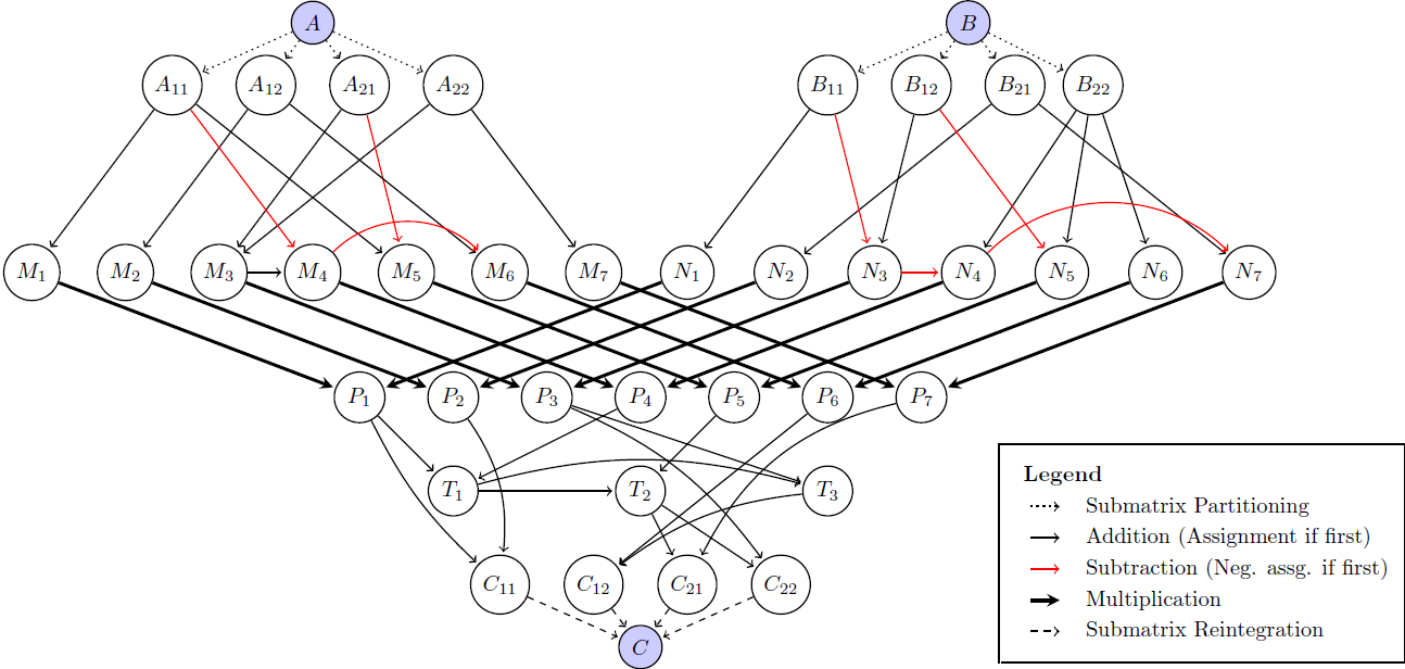
Example 2.36. Strassen’s Algorithm.
Standard multiplication of two
\(n\times n\) matrices requires about
\(n^3\) operations.
Strassen’s algorithm partitions matrices and reduces the complexity to approximately
\(n^{2.803}\text{.}\)
Example 2.37. Fast Fourier Transform.
The Fast Fourier Transform (FFT) is another algorithm that uses partitioned matrices recursively.
\begin{equation*}
G_0 =
\begin{bmatrix}1\end{bmatrix},
\qquad
G_{n+1} =
\begin{bmatrix}
G_n \amp -G_n\\
G_n \amp G_n
\end{bmatrix}.
\end{equation*}
This recursive structure allows computation in nearly linear time, a dramatic improvement over
\(n^3\text{.}\)