Section 1.3 Vector Equations

Handout 1.3 Vector Equations

We want to think about the algebra in linear algebra (systems of equations and their solution sets) in terms of geometry (points, lines, planes, etc.). Consider the following system.
\begin{equation*} \begin{aligned} x - 3y \amp = -3\\ 2x + y \amp = 8 \end{aligned} \end{equation*}
We could solve this system by graphing the lines represented by each equation and determining where they interesect.
Two lines intersecting in the plane in a single point.
Cartesian axes with two lines: one with positive slope (from the equation \(x-3y=-3\)) and one with negative slope (from \(2x+y=8\)), intersecting at a point.
Figure 1.21. Two lines in the plane with a single point of intersection.
This geometric perspective gives better insight into properties of systems and their solution sets. To better see this, we introduce \(n\)-dimensional space \(\mathbb{R}^n\) and the vectors that live in it.

Definition 1.22.

Recall that \(\mathbb{R}\) denotes the collection of all real numbers. For a positive integer \(n\text{,}\) define
\begin{equation*} \mathbb{R}^n = \{\text{all ordered } n\text{-tuples of real numbers } (x_1,\,x_2,\,\ldots,\,x_n)\}. \end{equation*}
When \(n=1\text{,}\) we get \(\mathbb{R}^1=\mathbb{R}\text{,}\) the number line.
A horizontal line with tick marks labeled from -3 to 3 representing the real number line.
Figure 1.23. The number line for \(\mathbb{R}\text{.}\)
When \(n=2\text{,}\) we can think of \(\mathbb{R}^2\) as a plane. Each point is an ordered pair of real numbers: its \(x\)- and \(y\)-coordinates. We could also view the elements of \(\mathbb{R}^n\) as vectors (arrows with length and direction). It turns out, viewing them as vector is a better approach.

Example 1.24.

Sketch the point \((3,2)\) and the vector \(\begin{bmatrix}3\\ 2\end{bmatrix}\text{.}\)
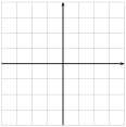
A square grid with horizontal and vertical axes spanning from -4 to 4.
Figure 1.25. Cartesian plane with grid and axes.
Answer.
The point \((3,2)\) should be a dot at the location in the grid with \(x\)-value 3 and \(y\)-value 2. The vector \(\begin{bmatrix} 3 \\ 2 \end{bmatrix}\) should be a ray with tail (or starting positing) at the origin and head (or ending positing with arrow) at the point \((3,2)\text{.}\)
When we think of an element of \(\mathbb{R}^n\) as a vector, we commonly write it as a column:
\begin{equation*} \vec v \;=\; \begin{bmatrix} 1\\ 2\\ 3 \end{bmatrix} \in \mathbb{R}^3. \end{equation*}
Suppose \(c\) is an arbitrary real number, written \(c \in \mathbb{R}\text{,}\) and let
\begin{equation*} \vec u \;=\; \begin{bmatrix} u_1\\ u_2 \end{bmatrix} \in \mathbb{R}^2, \qquad \vec v \;=\; \begin{bmatrix} v_1\\ v_2 \end{bmatrix} \in \mathbb{R}^2. \end{equation*}
Vectors have the following properties.
  1. Scalar Multiple:
    \begin{equation*} c\,\vec u \;=\; \begin{bmatrix} c\,u_1\\ c\,u_2 \end{bmatrix}. \end{equation*}
  2. Vector Addition:
    \begin{equation*} \vec u + \vec v \;=\; \begin{bmatrix} u_1\\ u_2 \end{bmatrix} + \begin{bmatrix} v_1\\ v_2 \end{bmatrix} \;=\; \begin{bmatrix} u_1 + v_1\\ u_2 + v_2 \end{bmatrix}. \end{equation*}
Vectors in higher dimensions satisfy the same operations componentwise.
Solution.
Some examples:
  • Let \(\vec u = \begin{bmatrix} 1 \\ 3 \end{bmatrix}\) and \(c = 2\)
    Then \(c\vec u = 2\begin{bmatrix} 1 \\ 3 \end{bmatrix} = \begin{bmatrix} 2(1) \\ 2(3) \end{bmatrix} = \begin{bmatrix} 2 \\ 6 \end{bmatrix}\)
    If \(d = -1\text{,}\) then \(d\vec u = -1\begin{bmatrix} 1 \\ 3 \end{bmatrix} = \begin{bmatrix} -1 \\ -3 \end{bmatrix}\)
    Geometrically, multiplying by the scalar \(c\in\mathbb{R}\) scales the vector by \(|c|\) and rotates the vector about the origin by 180 degrees if \(c < 0\text{.}\)
  • Let \(\vec u = \begin{bmatrix} 1 \\ 2 \end{bmatrix}\) and \(\vec v = \begin{bmatrix} -2 \\ 1 \end{bmatrix}\)
    Then \(\vec u + \vec v = \begin{bmatrix} 1 \\ 2 \end{bmatrix} + \begin{bmatrix} -2 \\ 1 \end{bmatrix} = \begin{bmatrix} 1 - 2 \\ 2 + 1 \end{bmatrix} = \begin{bmatrix} -1 \\ 3 \end{bmatrix}\)
    Geometrically, vector addition follows the parallelogram rule. This means that to sketch the vector \(\vec u + \vec v\text{,}\) you first sketch the vector \(\vec u\) starting from the origin. Then, you sketch the vector \(\vec v\) starting from the head of \(\vec u\text{.}\) The vector \(\vec u + \vec v\) is the drawn by starting at the origin and ending where \(\vec v\) ended.
  • Vectors with a different number of entries cannot be added together.
    \(\begin{bmatrix} 1 \\ 2 \end{bmatrix} + \begin{bmatrix} 1 \\ 2 \\ 3 \end{bmatrix}\) is not defined.

Definition 1.26.

  1. Given vectors \(\vec v_1,\vec v_2,\dotsc,\vec v_p \in \mathbb{R}^n\) and scalars \(c_1,c_2,\dotsc,c_p\text{,}\) the vector
    \begin{equation*} \vec y \;=\; c_1 \vec v_1 + c_2 \vec v_2 + \cdots + c_p \vec v_p \end{equation*}
    is called a linear combination of \(\vec v_1,\dotsc,\vec v_p\) with weights \(c_1,\dotsc,c_p\text{.}\)
  2. The set of all linear combinations of \(\vec v_1,\dotsc,\vec v_p\) is called the span of these vectors.
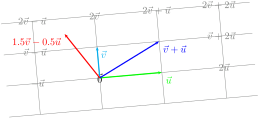
Any two vectors in \(\mathbb{R}^2\) that are not scalar multiples of one another span \(\mathbb{R}^2\text{.}\) Thus, any vector in \(\mathbb{R}^2\) can be written as a linear combination of such a pair.
A grid representing the span of two linearly independent vectors
A lightly rotated square grid with the origin and multiples/sums of two non-parallel vectors labeled, illustrating how combinations like \(\vec v+\vec u\text{,}\) \(2\vec v+\vec u\text{,}\) etc., tile the plane.
Figure 1.27. Linear combinations of two nonparallel vectors spanning the plane.

Example 1.28.

Let \(\vec u=\begin{bmatrix} -1\\ 4\\ 2\end{bmatrix}\) and \(\vec v=\begin{bmatrix} 5\\ 0\\ -3\end{bmatrix}\text{.}\) Determine three vectors which are linear combinations of \(\vec u\) and \(\vec v\text{.}\)
Solution.
The following are linear combinations \(\vec u\) and \(\vec v\text{.}\)
  • \(\displaystyle 3\vec u + 5\vec v = \begin{bmatrix} -3 \\ 12 \\ 6 \end{bmatrix} + \begin{bmatrix} 25 \\ 0 \\ -15 \end{bmatrix} = \begin{bmatrix} 22 \\ 12 \\ -9 \end{bmatrix}\)
  • \(\displaystyle 0\vec u + (-3)\vec v = \begin{bmatrix} -15 \\ 0 \\ 9 \end{bmatrix}\)
  • \(\displaystyle 0\vec u + 0\vec v = \begin{bmatrix} 0 \\ 0 \\ 0 \end{bmatrix} = \vec 0\)
So, we have that \(\begin{bmatrix} 22 \\ 12 \\ -9 \end{bmatrix}, \begin{bmatrix} -15 \\ 0 \\ 9 \end{bmatrix}, \vec 0 \in \operatorname{Span}\left\{\vec u, \vec v\right\}\)

Example 1.29.

Let \(\vec u=\begin{bmatrix} -1\\ 4\\ 2\end{bmatrix}\) and \(\vec v=\begin{bmatrix} 5\\ 0\\ -3\end{bmatrix}\text{.}\) Determine if \(\vec w = \begin{bmatrix} 2 \\ 12 \\ 3 \end{bmatrix}\) is in \(\operatorname{Span}(\vec u, \vec v)\text{.}\)
Solution.
Note that \(\vec w \in\operatorname{Span}\{\vec u, \vec v\}\) if and only if \(\vec w\) can be written as a linear combination of the vectors \(\vec u\) and \(\vec v\text{;}\) that is, if and only if there exist \(c_1, c_2 \in \mathbb{R}\) so that
\begin{equation*} c_1\vec u + c_2 \vec v = \vec w \iff \begin{bmatrix}-c_1 + 5c_2 \\ 4c_1 \\ 2c_1 - 3c_2 \end{bmatrix} = \begin{bmatrix} 2 \\ 12 \\ 3 \end{bmatrix} \end{equation*}
Note that this leads to the following system of linear equations:
\begin{equation*} \left\{\begin{array}{rrrrr} -c_1 \amp + \amp 5c_2 \amp = \amp 2 \\ 4c_1 \amp \amp \amp = \amp 12 \\ 2c_1 \amp - \amp 3c_2 \amp = \amp 3 \end{array}\right. \end{equation*}
We will determine if this system has a solution by row reducing the corresponding augmented matrix. Note that
\begin{equation*} \begin{bmatrix} -1 \amp 5 \amp \rvert \amp 2 \\ 4 \amp 0 \amp \rvert \amp 12 \\ 2 \amp -3 \amp \rvert \amp 3 \end{bmatrix} \sim \begin{bmatrix}1 \amp -5 \amp \rvert \amp -2 \\ 0 \amp 20 \amp \rvert \amp 20 \\ 0 \amp 7 \amp \rvert \amp 7 \end{bmatrix} \sim \begin{bmatrix} 1 \amp 0 \amp \rvert \amp 3 \\ 0 \amp 1 \amp \rvert \amp 1 \\ 0 \amp 0 \amp \rvert \amp 0 \end{bmatrix} \end{equation*}
It follows that the system has the solution \(c_1 = 3\) and \(c_2 = 1\text{.}\) Therefore, we have that
\begin{equation*} \vec w = 3\vec u + 1\vec v \in \operatorname{Span}\{\vec u, \vec v\} \end{equation*}
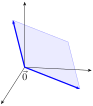
In general, any two non-parallel vectors in \(\mathbb{R}^3\) span a plane through the origin. Every vector in that plane is a linear combination of the two.
A translucent plane through the origin with two nonparallel vectors drawn from the origin; coordinate axes are shown for reference.
Figure 1.30. Two nonparallel vectors in \(\mathbb{R}^3\) span a plane through the origin.

Example 1.31.

Is \(\vec y\) in the span of \(\vec v_1\) and \(\vec v_2\text{?}\)
\begin{equation*} \vec v_1 \;=\; \begin{bmatrix} 1\\ -2\\ -3 \end{bmatrix},\qquad \vec v_2 \;=\; \begin{bmatrix} 2\\ 5\\ 6 \end{bmatrix},\qquad \vec y \;=\; \begin{bmatrix} 7\\ 4\\ 15 \end{bmatrix}. \end{equation*}
Solution.
Similar to ExampleΒ 1.29, we form the augmented matrix \(\begin{bmatrix} \vec v_1 \amp \vec v_2 \amp \rvert \amp \vec y \end{bmatrix}\) and determine if there are any solutions. Note the following: \(\begin{eqnarray*} \begin{bmatrix} \vec v_1 \amp \vec v_2 \amp \rvert \amp \vec y \end{bmatrix} \amp = \amp \begin{bmatrix} 1 \amp 2 \amp \rvert \amp 7 \\ -2 \amp 5 \amp \rvert \amp 4 \\ -3 \amp 6 \amp \rvert \amp 15 \end{bmatrix} \\ \amp \sim \amp \begin{bmatrix} 1 \amp 2 \amp \rvert \amp 7 \\ 0 \amp 9 \amp \rvert \amp 18 \\ 0 \amp 12 \amp \rvert \amp 36 \end{bmatrix} \\ \amp \sim \amp \begin{bmatrix} 1 \amp 2 \amp \rvert \amp 7 \\ 0 \amp 1 \amp \rvert \amp 2 \\ 0 \amp 1 \amp \rvert \amp 3 \end{bmatrix}\\ \amp \sim \amp \begin{bmatrix} 1 \amp 2 \amp \rvert \amp 7 \\ 0 \amp 1 \amp \rvert \amp 2 \\ 0 \amp 0 \amp \rvert \amp 1 \end{bmatrix} \end{eqnarray*}\)
It follows that the system is inconsistent. Therefore, it is impossible to express \(\vec y\) as a linear combination of \(\vec v_1\) and \(\vec v_2\text{.}\) Thus,
\begin{equation*} \vec y \not\in \operatorname{Span}\{\vec v_1,\vec v_2\}\text{.} \end{equation*}