Skip to main content
Contents Embed Dark Mode Prev Up Next \(\newcommand{\foo}{b^{ar}}
\newcommand{\aug}{\fboxsep=-\fboxrule\!\!\!\fbox{\strut}\!\!\!}
\newcommand{\Nul}{\operatorname{Nul}}
\newcommand{\Col}{\operatorname{Col}}
\newcommand{\Row}{\operatorname{Row}}
\newcommand{\Span}{\operatorname{Span}}
\renewcommand{\det}{\operatorname{det}}
\newcommand{\rank}{\operatorname{rank}}
\newcommand{\proj}{\operatorname{proj}}
\newcommand{\dist}{\operatorname{dist}}
\newcommand{\lt}{<}
\newcommand{\gt}{>}
\newcommand{\amp}{&}
\definecolor{fillinmathshade}{gray}{0.9}
\newcommand{\fillinmath}[1]{\mathchoice{\colorbox{fillinmathshade}{$\displaystyle \phantom{\,#1\,}$}}{\colorbox{fillinmathshade}{$\textstyle \phantom{\,#1\,}$}}{\colorbox{fillinmathshade}{$\scriptstyle \phantom{\,#1\,}$}}{\colorbox{fillinmathshade}{$\scriptscriptstyle\phantom{\,#1\,}$}}}
\)
Section 1.1 Systems of Linear Equations
Handout 1.1 Systems of Linear Equations
Objectives: Topics
Systems of Linear Equations
Matrix Notation
Elementary Row Operations
Existence and Uniqueness of Solutions
Objectives: Goals
Characterize a linear system by the number of solutions and consistency.
Apply elementary row operations to solve linear systems.
Express a system as an augmented matrix.
Definition 1.1 . A Single Linear Equation.
A linear equation has the form:
\begin{equation*}
a_1 x_1 + a_2 x_2 + \cdots + a_n x_n = b
\end{equation*}
where, \(a_1,\dots,a_n\) and \(b\) are the coefficients , \(x_1,\dots,x_n\) are the variables (unknowns), and \(n\) is the dimension (number of variables).
Some Examples:
\(2x_1+4x_2=4\) is a line in two dimensions.
\(3x_1+2x_2+x_3=6\) is a plane in three dimensions.
\(\displaystyle x_1 + x_2 + x_3 = x_4 + x_5\)
\(\displaystyle x_1 + \sqrt{2}x_2 -\frac{1}{7} = \pi x_3\)
Non Examples:
\(\displaystyle x_1 + x_2^3 = 3\)
\(\displaystyle 2x_1 - 4x_2 - \sqrt{x_3} = 4\)
\(\displaystyle \dfrac{1}{x_1} + x_2 + x_3 = 4\)
\(\displaystyle \sin(x_1) + x_2 = 3\)
When we have more than one linear equation, we have a
system of linear equations . For example, a system of two linear equations is:
\begin{equation*}
\begin{aligned}
x_1 \amp\;+\; 1.5\,x_2 \;+\; \pi x_3 \;=\; 4 \\
5x_1 \amp\;+\; \phantom{1.5\,x_2}\;+\; 7x_3 \;=\; 5
\end{aligned}
\end{equation*}
Definition 1.2 . Solution to a Linear System.
The set of all possible values of \(x_1, x_2, \ldots, x_n\) that satisfy every equation in the system is the solution, or solution set, to the system.
Solution .
Consider finding solutions to the system given
above . At this point, we don’t have a great way of determining the solutions to a system of linear equations. We can try guessing some solutions.
Try \((4,0,0)\text{:}\) Note this points makes the first equation true since \(4 + 1.5(0) + \pi(0) = 4\text{,}\) but it does not make the second equation true since \(5(4) + 7(0) \neq 5\text{.}\) Therefore, \((4,0,0)\) is not a solution to the system.
Try \((1,2,0)\text{:}\) Note plugging this point into the first equation yields \(1 + 1.5(2) + \pi(0) = 4\) which is a true statement. Plugging the point into the second equation yields \(5(1) + 7(0) = 5\) which is also a true statement. Since the point makes both equations true, it is a solution to the system.
Can you find any more solutions?
How many solutions can a system have?
Example 1.3 .
Consider the following systems of two linear equations in two variables and determine how many solutions there are for each.
(a) \(\begin{aligned}
x_1 - 2x_2 \amp= -1 \\
-x_1 + 3x_2 \amp= \phantom{-}3
\end{aligned}\) Solution .
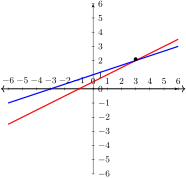
Graphing the two lines gives the following:
The graph of the lines \(x_1 - 2x_2 = -1\) (in red) and \(-x_1 + 3x_2 = 3\) (in blue), showing their intersection point at \((3,2)\)
Figure 1.4. Two lines in the plane with a single point of intersection. We see that the lines only intersect at
\((3,2)\text{,}\) so this is the only solution to the system.
(b) \(\begin{aligned}
x_1 - 2x_2 \amp= -1 \\
-x_1 + 2x_2 \amp= \phantom{-}3
\end{aligned}\) Solution .
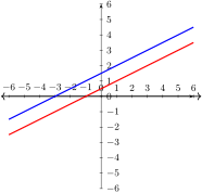
Graphing the two lines gives the following:
The graph of the lines \(x_1 - 2x_2 = -1\) (in red) and \(-x_1 + 2x_2 = 3\) (in blue)
Figure 1.5. Two parallel lines in the plane. We see that the lines are parallel, so they never intersect. Therefore, there is no solution to the system.
(c) \(\begin{aligned}
x_1 - 2x_2 \amp= -1 \\
-x_1 + 2x_2 \amp= \phantom{-}1
\end{aligned}\) Solution .
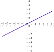
Graphing the two lines gives the following:
The graph of the lines \(x_1 - 2x_2 = -1\) (in red) and \(-x_1 + 2x_2 = 1\) (in blue)
Figure 1.6. Two lines lying on top of one another. The two linear equations give the same line. Therefore, there are infinitely many points that satisfy both equations, any point that is on the line.
Conclusion: A system of linear equations in two variables can have
\(\underline{\hspace{4in}}\) solutions.
Answer .
zero, one, or infinitely many
A linear equation in three variables,
\(a_1x_1+a_2x_2+a_3x_3=b\text{,}\) defines a plane in
\(\mathbb{R}^3\text{.}\)
Example 1.7 .
How many solutions can a system of
two linear equations in three variables have?
Hint .
Play around with drawing two planes in 3-space and seeing how they intersect. Can they never intersect? What about intersect in a finite number of points? What about intersect in infinitely many points?
Answer .
zero or infinitely many. It is
impossible to have exactly one solution in this case.
Example 1.8 .
How many solutions can a system of
three linear equations in three variables have?
Hint .
Play around with drawing three planes in 3-space and seeing how they intersect. Can they never intersect? What about intersect in a finite number of points? What about intersect in infinitely many points?
Answer .
zero, one, or infinitely many
Conclusion: Every system of linear equations, no matter the number of equations and number of variables has
\(\underline{\hspace{4in}}\) solutions.
Answer .
zero, one, or infinitely many
As we saw in the previous examples, one way to solve a system of linear equations is by graphing. This is not practical for most examples, especially if we are working with four or more varialbes. A more useful approach to solving a linear system is to manipulate the equations through the use of
row operations .
Replacement/Addition: add a multiple of one row to another.
Interchange: swap two rows.
Scaling: multiply a row by a nonzero scalar.
Example 1.9 .
Apply row operations to systematically simplify the system below to an equivalent (easier to read) form in order to more easily identify the solution(s).
\begin{alignat*}{4}
x_1 \amp {}-{} \amp 2x_2 \amp {}+{} \amp x_3 \amp {}={} \amp 0 \\
\amp \amp 2x_2 \amp {}-{} \amp 8x_3 \amp {}={} \amp 8 \\
5x_1 \amp \amp \amp {}-{} \amp 5x_3 \amp {}={} \amp 10
\end{alignat*}
Solution .
We will simplify the system using appropriate row operations. I am going to go ahead and use augmented matrices since that is what we will do from here on out.
\(\begin{eqnarray*}\begin{bmatrix} 1 \amp -2 \amp 1 \amp \rvert \amp 0 \\ 0 \amp 2 \amp -8 \amp \rvert \amp 8 \\ 5 \amp 0 \amp -5 \amp \rvert \amp 10 \end{bmatrix} \amp \overset{R_3-5R_1 \rightarrow R_3}{\Huge \sim} \amp \begin{bmatrix} 1 \amp -2 \amp 1 \amp \rvert \amp 0 \\ 0 \amp 2 \amp -8 \amp \rvert \amp 8 \\ 0 \amp 10 \amp -10 \amp \rvert \amp 10 \end{bmatrix} \\
\amp \overset{\frac{1}{2}R_2 \rightarrow R_2}{\underset{\frac{1}{10}R_3 \rightarrow R_3}{\Huge \sim}} \amp \begin{bmatrix} 1 \amp -2 \amp 1 \amp \rvert \amp 0 \\ 0 \amp 1 \amp -4 \amp \rvert \amp 4 \\ 0 \amp 1 \amp -1 \amp \rvert \amp 1\end{bmatrix} \\
\amp \overset{R_1 + 2R_2 \rightarrow R_1}{\underset{R_3 - R_2 \rightarrow R_3}{\Huge \sim}} \amp \begin{bmatrix}1 \amp 0 \amp -7 \amp \rvert \amp 8 \\ 0 \amp 1 \amp -4 \amp \rvert \amp 4 \\ 0 \amp 0 \amp 3 \amp \rvert \amp -3 \end{bmatrix} \\
\amp \overset{\frac{1}{3}R_3 \rightarrow R_3}{\Huge \sim} \amp \begin{bmatrix} 1 \amp 0 \amp -7 \amp \rvert \amp 8 \\ 0 \amp 1 \amp -4 \amp \rvert \amp 4 \\ 0 \amp 0 \amp 1 \amp \rvert \amp -1 \end{bmatrix} \\
\amp \overset{R_1 + 7R_3 \rightarrow R_1}{\underset{R_2 + 4R_3 \rightarrow R_2}{\Huge \sim}} \amp \begin{bmatrix} 1 \amp 0 \amp 0 \amp \rvert \amp 1 \\ 0 \amp 1 \amp 0 \amp \rvert \amp 0 \\ 0 \amp 0 \amp 1 \amp \rvert \amp -1 \end{bmatrix}
\end{eqnarray*}\)
Therefore, we have that the only solution is
\((1,0,-1)\text{.}\)
It’s redundant to write variables repeatedly, so we use a augmented matrix to simplify the notation for the system. For example, the previous system
\begin{alignat*}{4}
x_1 \amp {}-{} \amp 2x_2 \amp {}+{} \amp x_3 \amp {}={} \amp 0 \\
\amp \amp 2x_2 \amp {}-{} \amp 8x_3 \amp {}={} \amp 8 \\
5x_1 \amp \amp \amp {}-{} \amp 5x_3 \amp {}={} \amp 10
\end{alignat*}
Can be writen as the augmented matrix
\begin{equation*}
\left[\begin{array}{rrr|r}
1 \amp -2 \amp 1 \amp 0 \\
0 \amp 2 \amp -8 \amp 8 \\
5 \amp 0 \amp -5 \amp 10
\end{array}\right]
\end{equation*}
The vertical bar separates the coefficient matrix (for \(x_1,x_2,x_3\) ) from the constants.
Example 1.10 .
Determine if the following system has a solution.
\begin{alignat*}{4}
\amp \amp x_2 \amp {}-{} \amp 4x_3 \amp {}={} \amp 8 \\
2x_1 \amp {}-{} \amp 3x_2 \amp {}+{} \amp 2x_3 \amp {}={} \amp 1 \\
4x_1 \amp {}-{} \amp 8x_2 \amp {}+{} \amp 12x_3 \amp {}={} \amp 1
\end{alignat*}
Solution .
\(\begin{eqnarray*}
\begin{bmatrix}
0 \amp 1 \amp -4 \amp \rvert \amp 8 \\
2 \amp -3 \amp 2 \amp \rvert \amp 1 \\
4 \amp -8 \amp 12 \amp \rvert \amp 1
\end{bmatrix} \amp \overset{\frac{1}{4}R_3 \rightarrow R_3}{\Huge \sim} \amp \begin{bmatrix}
0 \amp 1 \amp -4 \amp \rvert \amp 8 \\
2 \amp -3 \amp 2 \amp \rvert \amp 1 \\
1 \amp -2 \amp 3 \amp \rvert \amp \frac{1}{4}
\end{bmatrix}
\\[1em]
\amp \overset{\text{swap } R_1 \text{ and } R_3}{\Huge \sim} \amp \begin{bmatrix}
1 \amp -2 \amp 3 \amp \rvert \amp \frac{1}{4} \\
2 \amp -3 \amp 2 \amp \rvert \amp 1 \\
0 \amp 1 \amp -4 \amp \rvert \amp 8
\end{bmatrix}
\\[1em]
\amp \overset{R_2 - 2R_1 \rightarrow R_2}{\Huge \sim} \amp \begin{bmatrix}
1 \amp -2 \amp 3 \amp \rvert \amp \frac{1}{4} \\
0 \amp 1 \amp -4 \amp \rvert \amp \frac{1}{2} \\
0 \amp 1 \amp -4 \amp \rvert \amp 8
\end{bmatrix}
\\[1em]
\amp \overset{R_3 - R_2 \rightarrow R_3}{\Huge \sim} \amp \begin{bmatrix}
1 \amp -2 \amp 3 \amp \rvert \amp \frac{1}{4} \\
0 \amp 1 \amp -4 \amp \rvert \amp \frac{1}{2} \\
0 \amp 0 \amp 0 \amp \rvert \amp \frac{15}{2}
\end{bmatrix}
\end{eqnarray*}\)
Note that the final row suggests that
\(0 = \frac{15}{2}\) which is impossible, no matter the choice of
\(x_1, x_2, x_3\text{.}\) Therefore, there is no solution. So the system is inconsistent.
Definition 1.11 . Consistent.
A linear system is consistent if it has at least one solution . Otherwise, it is inconsistent .
Definition 1.12 . Row Equivalence.
Two matrices are row equivalent if a sequence of row operations transforms one matrix into the other.
Note : If the augmented matrices of two linear systems are row equivalent, they have the same solution set.
Fundamental Questions : Two questions that we will revisit many times throughout the course:
Does a given linear system have a solution? In other words, is it consistent?
If it is consistent, is the solution unique?